Introduction to Autoencoders and Common Issues and Challenges

What are Autoencoders?

An autoencoder is an artificial neural deep network that uses unsupervised machine learning. It is an efficient learning procedure that can encode and also compress data using neural information processing systems and neural computation. Then it is able to take that compressed or encoded data and reconstruct it in a way that is as close to the original input as possible.

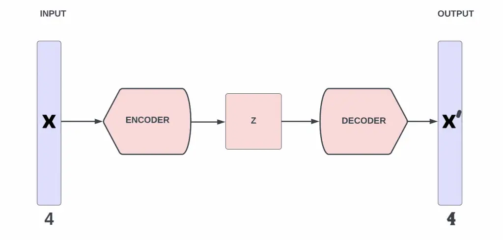
Autoencoders by design are able to learn how to ignore noise in data, thus reducing data dimensions. In a data set, noise refers to any data that is meaningless or corrupt. Autoencoders are able to take on the ImageNet Large Scale Recognition Challenge, where the goal is to classify a single image into 1000 different categories using imagenet classification. There are four main components to the autoencoder process and they can be seen below:

1. The first main component of an autoencoder is the encoder. This is where the model first learns how to compress the inputted data and encode it by reducing the dimensions of the data. The data set produced from this then becomes the benchmark dataset. It does not matter if the input is high dimensional data, it can still be reduced.
2. The second main component is the bottleneck. This layer of the autoencoder houses the compressed version of the data. The data that is stored here is the lowest possible dimensional form of the input data.
3. The third component is the decoder. This is the opposite of the encoder. This is where the model learns how to reconstruct the compressed or encoded data back into the original input data.
4. The final component in an autoencoder is reconstruction loss. This is the part where the decoder’s data output is compared against the original data to see how close it is. The training method used here is back propagation and training metrics. Back-propagation is the essence of neural net training. It is the practice of fine-tuning the weights of a neural net based on the error rate obtained in the previous iteration.This error rate can be determined using contrastive divergence learning.
   

Variational Autoencoder

Now that we know how autoencoders function, let’s look at one type of autoencoder called variational autoencoder. A variational autuencoder is a deep learning generative graphical model. Deep generative models have shown an incredible ability to produce highly realistic pieces of content of various kind, such as images, texts, and sounds.

A variational autoencoder is one that is trained to avoid overfitting and ensure that the latent space can enable the generative process. Overfitting is a concept in data science, which occurs when a statistical model fits exactly against its training data. When this happens, the algorithm unfortunately cannot perform accurately against unseen data, defeating its purpose. In an autoencoder, the latent space is part of the decoder. The lower-dimensional space in the middle of the decoder is known as the latent space.

The variational autoencoder is slightly different from an autoencoder. Although it has an encoder and a decoder. They are both trained minimize the reconstruction error between the initial data and the decoded data, which is similar to a normal autoencoder. However there is a slight change because the latent space needs to be regularized during the encoding and decoding process. Instead of encoding an input as a single point, we encode it as a distribution over the latent space. The full process can be seen below:

1. In the first step we have to take the input and encode it as a distribution over a latent space, not the original space. The encoder in this case is learning to approximate the posterior distribution of the data.
   
2. In the second step we have to first choose a single point from the latent space that was sampled from the distribution.
3. For the third step the chosen sampled point from step two is decoded. Then the reconstruction error is calculated on this decoded output.
4. Finally, in the fourth step the reconstruction error is back propagated throughout the network.

We talk a lot about regularization, but what does it mean? Well when we say the latent space should be regular, that means it needs to be both continuous and complete. Continuity means two close points in the latent space should not give two completely different contents once decoded. Completeness means for a chosen distribution, a point sampled from the latent space should give meaningful content once decoded.To learn how to build a keras variational autoencoder you can visit their website here.

Under Complete Autoencoder

Out of all the different types of autoencoders, the under complete autoencoder is the most simple and easiest to understand. The way it functions is very straightforward. The objective of an under complete autoencoder is to capture the most important features present in the data using representation learning. Under complete autoencoders have a smaller dimension for the hidden layer compared to the visible layer. This helps to obtain important features from the data.

An under complete autoencoder functions by first taking in an image and then it tries to predict the same image as what would be the output. This is how it manages to reconstruct the image from the bottleneck region. Under complete autoencoders are unsupervised, meaning they do not need labeled data in order to function. One advantage of using an under complete autoencoder is Under complete autoencoders that they do not need any regularization as they maximize the probability of data rather than copying the input to the output.

One drawback to using under complete autoencoders is that they suffer from overfitting. Under complete autoencoders are mostly used to generate the bottleneck or latent space. Doing this helps to create a compressed version of the user inputted data. Ideally we want the under complete autoencoder to describe and learn the latent attributes of the input data. Under complete autoencoders can also be thought of as a more advanced method of principal components analysis.

Principal component analysis, or PCA, is a statistical procedure that allows you to summarize the information content in large data tables by means of a smaller set of summary indices that can be more easily visualized and analyzed. Unlike PCA though, the under complete autoencoder is able to find an even lower hyper-dimensional plane that is able to describe the data.

Sparse Autoencoder

A sparse autoencoder is one of a range of types of autoencoder artificial neural networks that work on the principle of unsupervised machine learning. Autoencoders seek to use items like feature selection and feature extraction to promote more efficient data coding.

Autoencoders often use a technique called backpropagation to change weighted inputs, in order to achieve dimensionality reduction, which in a sense scales down the input for corresponding results. A sparse autoencoder is one that has small numbers of simultaneously active neural nodes. Now that we have a general idea of what a sparse autoencoder is, lets look at more specifics. A sparse autoecoder, unlike other autoencoders, is one that trains itself with something called a sparsity penalty.

A sparsity penalty can be created in two possible ways. One way is L1 regularization, and the other is KL-divergence. Both of these are complex topics, so this article will only tough a little on L1 and L2 regularization. L1 and L2 are both referred to as penalty terms. The penalty term added by L1 is the coefficients that represent the absolute value of magnitude, while the L2 penalty term is the coefficients that represent the magnitude squared. More about L1 regularization and why it leads to sparsity can be found here.

Sparse autoencoders have hidden nodes greater than input nodes. Because of this, when reconstructing the loss function we suffer penalties within the hidden layer. This is to prevent the output layer from copying input data. This sparsity penalty that is applied on the hidden layer in addition to the reconstruction error actually helps to prevent overfitting. Sometimes the data may be an identity function which will return the same argument. When this happens, a sparse autoencoder cannot be used. Unlike an under complete autoencoder, the sparse autoencoder only uses active regions of the networks instead of the entire network.

One drawback of sparse autoencoders is that it is essential that the individual nodes of a trained model which activate must be data dependent. This means that different inputs must result in activations of different nodes through the network. Some of the most powerful Artificial intelligence systems in the 2010s involved sparse autoencoders stacked inside of deep neural networks.

Also Read: What is a Sparse Matrix? How is it Used in Machine Learning?

Denoising Autoencoder

A denoising autoencoder is an autoencoder that is able to reconstruct data that was corrupted. A general autoencoder is designed in a way to perform feature selection and extraction using feature vectors. However it misses that the nodes that are in the hidden layer outnumber the inputs. This can lead to the situation called the null function, where the outputs equal the input, which makes the autoencoder seem useless. Denoising autoencoders are able to solve this issue.

Denoising autoencoders create a corrupted copy of the input by introducing some noise. This helps to avoid the autoencoders to copy the input to the output without learning features about the data. These autoencoders take a partially corrupted input while training to recover the original non distorted input. The model learns a vector field for mapping the input data towards a lower dimensional manifold which describes the natural data to cancel out the added noise.

What do we mean by corrupting the data though? Well this simply means turning some of the inputs to zero. The amount of inputs turned to zero can vary. Sometimes it may be 20%, other times it may even be 50%. Generally the amount will depend on the amount of data in the data set. To learn how to build a denoising autoencoder model you can visit this website.

There are some advantages to using denoising autoencoders. First, it minimizes the loss function between the output node and the corrupted input. Also setting up single thread denoising autoencoders is an easy process compared to other types of autoencoders. One drawback on this type of autoencoder is that it isn’t able to develop a mapping system which memorizes the training data because our input and target output are no longer the same. Another drawback is the training process that goes into denoising autoencoders. In order to train the model we first have to perform preliminary stochastic mapping in order to corrupt the data and use as input, this can increase the time it takes for the model to learn the object. Denoising autoencoders are better at feature selection than weakly supervised classification models.

Contractive Autoencoder

Denoising autoencoders may be good at feature selection, however contractive autoencoders are even better at it as they take into account hierarchical representations. A contractive autoencoder is a deep learning technique that aids a neural network in identifying unlabeled data by using grandient based learning. This type of autoencoder was first proposed in 2011 in order to make a large amount of small changes to training data sets. Like denoising autoencoders, contractive autoencoders also use a penalty term to account for the loss function. The loss function for the error of parameter estimates can be seen below:

Robustness of the representation for the data is done by applying a penalty term to the loss function. Contractive autoencoder is another regularization technique just like sparse and denoising autoencoders. However, this regularization technique corresponds to the Frobenius norm of the Jacobian matrix of the encoder activation with respect to the input. The Frobenius norm of the Jacobian matrix for the hidden layer is calculated with respect to input and it is basically the sum of square of all elements. Let’s first look at how to calculate the Jacobian matrix for the hidden layer. The calculation can be seen below:

The goal of a Contractive Autoencoder is to reduce the representation’s sensitivity towards the training input data. If the penalty or regularization term comes out to be zero, then it means that as we change input values, we don’t observe any change on the learned hidden representations. However, if the value is very large, then the learned representation is unstable as the input values change. This means contractive autoencoders need a fit model. Contractive autoencoders are usually deployed as just one of several other autoencoder nodes, activating only when other encoding schemes fail to label a data point. This can be used on datasets for workflow recognition, however cannot be used on threefold datasets.

Also Read: Is deep learning supervised or unsupervised?

Data Generating Process

Now that we examined a few different types of autoencoders, let’s look at the data generating process since it is a dynamical system. For example, let’s imagine we want to generate the number five as an image. In an autoencoder this would be generated from the latent variable centroid. Now imagine that we want to again generate the number five as an image, but this time we do not want it to look the same as the original five image.

So this time, we would take the input image of five using multicamera task recognition, then add some random noise to it inside the latent space and then pass it through the convolutional neural network. Now we have an image of the number five that looks slightly different than the original. You may encounter this technique being used in video games models, such as plants or trees.

Inherently, this learning procedure used, leads to parameter distribution that causes similar parameters being clustered together in a latent space. The autoencoder is trained using a set of images, in our case images of the number five, to learn the mean and standard deviation in the latent space. This is what forms the data distribution. This is a general explanation of the data generating process that abstracts away the actual architecture of autoencoders, so let’s talk about the architecture of encoders next.

Also Read: What Are Word Embeddings?

The Architecture of Autoencoders

We discussed four main components in autoencoders, these are encoder, bottleneck, decoder, and reconstruction loss. Let’s look more in depth at the first three. An encoder is the module that takes the input data and compresses it into data that is several times smaller. Having multiple dimensional data gives way to the what is known as the blessing or sometimes curse of dimensionality. This is a problem relating to various phenomena that can arise when analyzing data that is multidimensional. The bottleneck is where the compressed information is all stored. This makes the bottleneck the most important part. The decoder is the module that takes the compressed data and returns it back to before it was encoded. The output of the decoder is then compared against a ground truth.

Now that we reviewed the general idea, let’s start by going a little more in depth about the encoder first. The encoder is able to compress data by using convolutional blocks and pooling modules. These compact data down until is able to fit into the bottleneck. As explained before the bottleneck is the most important part of the neural information processing system. It is also the smallest part of the neural network. It’s existence is to strictly limit the information that flows between the encoder and decoder. It will only allow vital information to pass through it.

Bottlenecks help us form a knowledge representation of images for imaging systems, also known as the input. The smaller a bottleneck is, the lower chance that overfitting will occur. However making it way too small will make it so very little information will be stored. Lastly, the decoder itself is made up convolutional and un-sampling blocks. These come together to reconstruct the output from the bottleneck. The decoder is able to build back the image using latent attributes along with pattern analysis and machine intelligence. Multilayer Perceptron also exists in autencoders. Multilayer perceptron consists of three layers which are the input layer, hidden layer, and output layer.

Applications of Autoencoders

Now that we know how autoencoders function and different types of them, let’s finally examine the applications of them. Below are a few cases where an autoencoder can be used:

Dimensionality Reduction.

This is done using an under complete autoencoder. Recall that in an under complete autoencoder, the hidden layer will be smaller than the input layer. We can force the network to learn important features by reducing the hidden layer size. Let’s look at a small snippet of python code that can perform dimensionality reduction using an under complete autoencoder as a training example.

#defining input placeholder for autoencoder model and networks for object detection
input_img = Input(shape=(784,))
# "enc_rep" is the encoded representation of the input
enc_rep = Dense(2000, activation='relu')(input_img)
enc_rep = Dense(500, activation='relu')(enc_rep)
enc_rep = Dense(500, activation='relu')(enc_rep)
enc_rep = Dense(10, activation='sigmoid')(enc_rep)

# "decoded" is the lossy reconstruction of the input from encoded representation
decoded = Dense(500, activation='relu')(enc_rep)
decoded = Dense(500, activation='relu')(decoded)
decoded = Dense(2000, activation='relu')(decoded)
decoded = Dense(784)(decoded)

# this model maps an input to its reconstruction
autoencoder = Model(input_img, decoded)

In this example we see image reconstruction using dimensionality reduction on the high dimensional features of the fashion MNIST data set. You can get the data set from this website. Furthermore, the rest of the python code for the under complete autoencoder can be found here.

Image Denoising.

Now that we looked at an application of an under complete autoencoder, lets now look at an application of a denoising autoencoder. This is a technique similar to that of hyperspectral imaging. When our image get corrupted or there is a bit of noise in it, we call this image a noisy image. To obtain proper information about the content of image, we need to perform image denoising and rich feature hierarchy.

To do this we have to define our autoencoder in a way to remove the noise of the image. Let’s look at an example of this in use. For this example we will be using the MNIST digit data set. Documentation of the data set can be found here.

This is just one dataset, others can be used for example a dataset for activity could be used. Once again, we will only show a small amount of the python code, specifically the part that defines the denoising autoencoder. This can be seen below.

Input_img = Input(shape=(28, 28, 1))

x1 = Conv2D(64, (3, 3), activation='relu', padding='same')(Input_img)
x1 = MaxPool2D( (2, 2), padding='same')(x1)
x2 = Conv2D(32, (3, 3), activation='relu', padding='same')(x1)
x2 = MaxPool2D( (2, 2), padding='same')(x2)
x3 = Conv2D(16, (3, 3), activation='relu', padding='same')(x2)
encoded = MaxPool2D( (2, 2), padding='same')(x3)

# decoding architecture
x3 = Conv2D(16, (3, 3), activation='relu', padding='same')(encoded)
x3 = UpSampling2D((2, 2))(x3)
x2 = Conv2D(32, (3, 3), activation='relu', padding='same')(x3)
x2 = UpSampling2D((2, 2))(x2)
x1 = Conv2D(64, (3, 3), activation='relu')(x2)
x1 = UpSampling2D((2, 2))(x1)
decoded = Conv2D(1, (3, 3), padding='same')(x1)

autoencoder = Model(Input_img, decoded)

This code will remove the noise in the data set and will allow us to see the images more clearly. The full code can be found here,  Image denoising can also be used on videos, this is called scale video classification benchmark.

Image Generation.

Variational autoencoders are a generative model that are able to generate images. This is the opposite of a discriminative model which draws boundaries in space using discriminative tasks. The idea is that given input images like images of face or scenery, the system will generate similar images. This type of autoencoder is used in the art and animation industry. It can generate new character animations. It can also be used to make fake human images using analysis of feature pooling to transform images.

Conclusion

In conclusion, we talked about what autoencoders are, the different types of them, and the applications of them. Most likely you have already encountered them without knowing, as they are used in things like facial recognition and anomaly detection using one shot learning, which are seen in movies and video games.

You may have also seen it used in other industrial tasks. The most important thing to know about autoencoders is their purpose, which is to reduce noise in data and focus only on the areas of real value using deep learning algorithms. There are some other types of autoencoders out there not mentioned in this article such as LSTM autoencoders and convolutional autoencoders, however we will leave that for you the reader to discover!

Thank you for reading this article.